Strategy Parameter Optimization
After developing a trading strategy, how do you find the best combination of conditions? The finlab.optimize module provides the sim_conditions() function to automatically test all condition combinations and visually compare performance, helping you identify the strongest strategy.
Why Strategy Optimization?
When developing trading strategies, we often have multiple screening conditions:
- Technical: Moving average crossovers, new highs, RSI indicators
- Fundamental: P/E ratio, revenue growth, profitability
- Institutional: Institutional buying, margin balance changes
Each condition alone may produce mediocre performance, but combining multiple conditions may yield unexpected results. Manually testing all combinations is extremely time-consuming; sim_conditions() automates this process.
Quick Start
Basic Example: All Combinations of 3 Conditions
Suppose we have 3 screening conditions:
from finlab import data
from finlab.backtest import sim
from finlab.optimize.combinations import sim_conditions

close = data.get("price:收盤價")
rev = data.get('monthly_revenue:當月營收')
營業利益成長率 = data.get('fundamental_features:營業利益成長率')

# Define 3 conditions
c1 = (close > close.average(20)) & (close > close.average(60))  # Technical: MA breakout
c2 = 營業利益成長率 > 0                                          # Fundamental: profit growth
c3 = rev.average(3) / rev.average(12) > 1.1                     # Fundamental: revenue acceleration

# Set exit condition
exits = close < close.average(20)

# Conditions dictionary, keys are condition names
conditions = {'c1': c1, 'c2': c2, 'c3': c3}

# Test all combinations
report_collection = sim_conditions(
    conditions=conditions,
    hold_until={'exit': exits, 'stop_loss': 0.1},  # Exit when below MA, 10% stop-loss
    resample='M',           # Monthly rebalancing
    position_limit=0.1,     # Max 10% per stock
    upload=False            # Don't upload to cloud
)
This code automatically tests the following 7 combinations:
c1(technical only)c2(profit growth only)c3(revenue acceleration only)c1 & c2(technical + profit growth)c1 & c3(technical + revenue acceleration)c2 & c3(profit growth + revenue acceleration)c1 & c2 & c3(all three conditions)
Visual Performance Comparison
1. Cumulative Return Line Chart
Compare the equity curves of each combination:
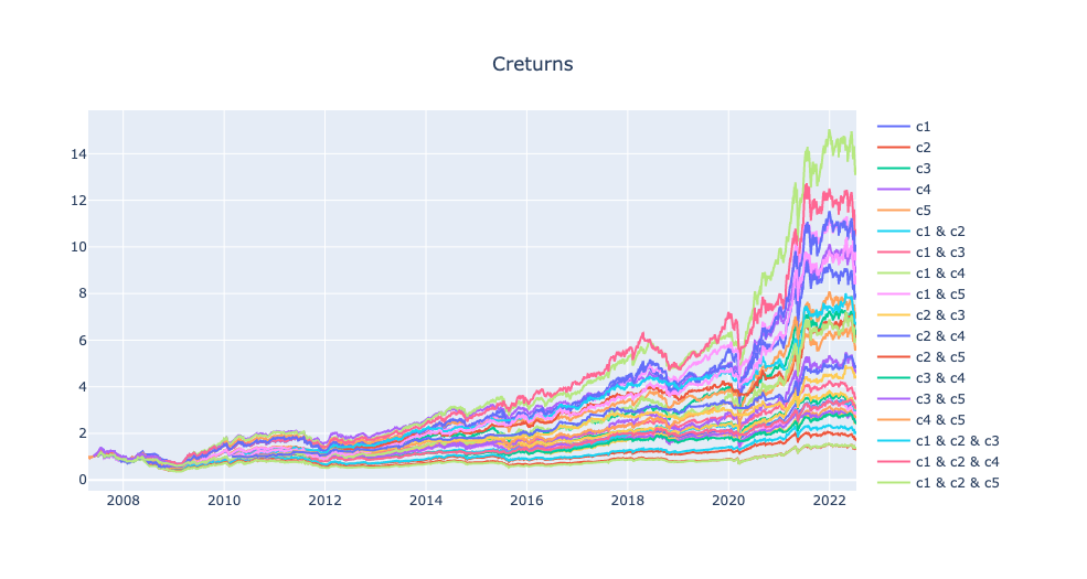
From the chart, you can see which combination has the best long-term performance and the stability of each combination.
2. Grouped Bar Chart of Metrics
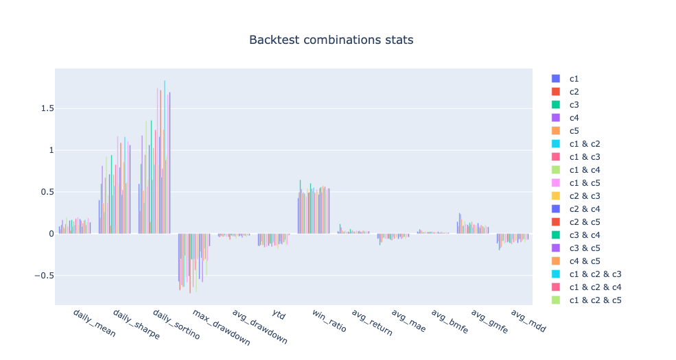
Displays 12 key metrics side by side for all combinations for quick comparison.
3. Metric Ranking Heatmap
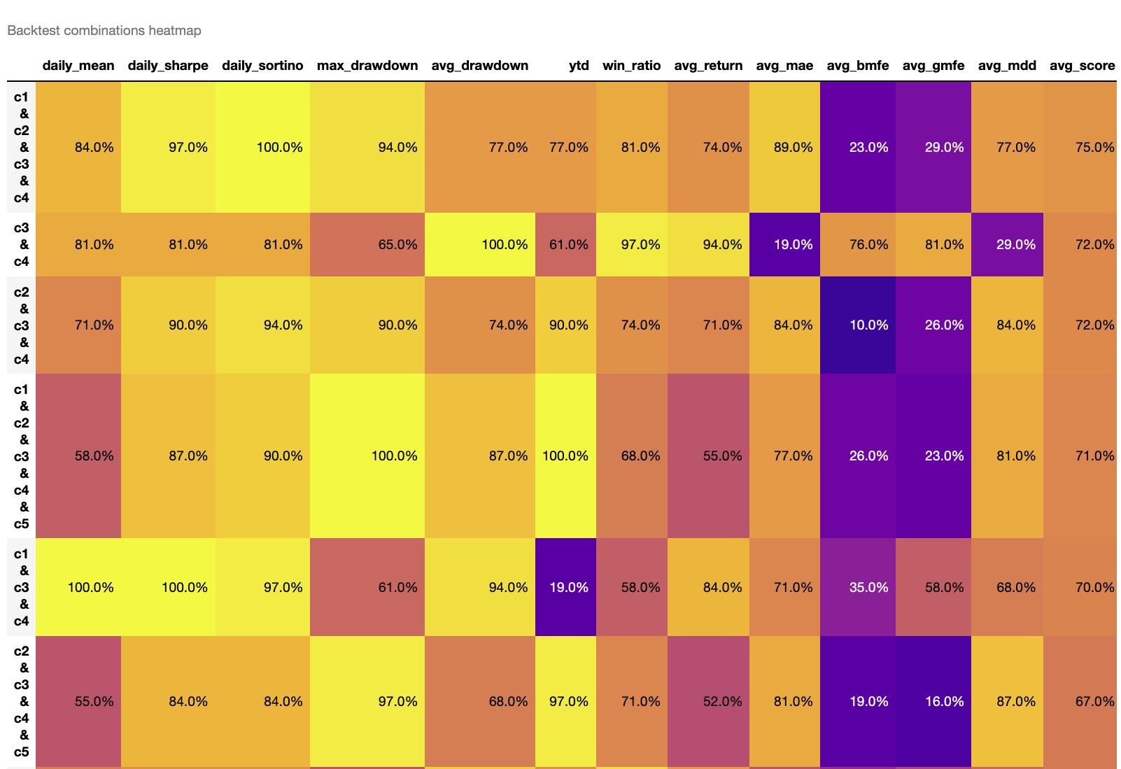
The heatmap uses color intensity to represent the percentile ranking (0-100%) of each metric. Higher values indicate better rankings:
- avg_score: Average score across all metrics; higher scores indicate better overall performance
- Sorted by
avg_scorein descending order by default, with the best combination at the top - Brighter colors (yellow) indicate higher rankings for that metric
How to interpret the heatmap
- Look for the combination with the highest avg_score (usually at the top)
- Check that the combination performs well on key metrics (Sharpe ratio, win rate, max drawdown)
- Avoid combinations with especially poor metrics (dark purple)
Get Detailed Performance Metrics
Returns a DataFrame with 12 metrics:
Strategy-Level Metrics
| Metric | Description | Direction |
|---|---|---|
daily_mean |
Annualized return | Higher is better |
daily_sharpe |
Annualized Sharpe ratio (risk-adjusted return) | Higher is better |
daily_sortino |
Annualized Sortino ratio (downside risk-adjusted return) | Higher is better |
max_drawdown |
Maximum drawdown (negative value) | Smaller absolute value is better |
avg_drawdown |
Average drawdown (negative value) | Smaller absolute value is better |
Trade-Level Metrics
| Metric | Description | Direction |
|---|---|---|
win_ratio |
Win rate per trade | Higher is better |
avg_return |
Average profit per trade | Higher is better |
avg_mae |
Average MAE per trade (negative value) | Smaller absolute value is better |
avg_bmfe |
Average BMFE (MFE before MAE) per trade | Higher is better |
avg_gmfe |
Average global MFE per trade | Higher is better |
avg_mdd |
Average max drawdown per trade (negative value) | Smaller absolute value is better |
Meaning of avg_bmfe
avg_bmfe represents how high the stock price went before the stop-loss was triggered. The higher this value, the more opportunity there is to take profit before the stop-loss -- an important reference for optimizing take-profit points.
Advanced Example: Optimization with 5 Conditions
When conditions increase to 5, the number of combinations reaches 31 (2^5 - 1). Manual testing is very difficult, but sim_conditions() handles it easily:
from finlab import data
from finlab.optimize.combinations import sim_conditions

close = data.get("price:收盤價")
pe = data.get('price_earning_ratio:本益比')
rev = data.get('monthly_revenue:當月營收').index_str_to_date()
rev_ma3 = rev.average(3)
rev_ma12 = rev.average(12)

# 5 conditions
c1 = (close > close.average(20)) & (close > close.average(60))  # MA bullish alignment
c2 = (close == close.rolling(20).max())                         # 20-day new high
c3 = pe < 15                                                    # Low P/E
c4 = rev_ma3 / rev_ma12 > 1.1                                   # Revenue acceleration
c5 = rev / rev.shift(1) > 0.9                                   # Monthly revenue change > -10%

exits = close < close.average(20)

conditions = {'c1': c1, 'c2': c2, 'c3': c3, 'c4': c4, 'c5': c5}

report_collection = sim_conditions(
    conditions=conditions,
    hold_until={'exit': exits, 'stop_loss': 0.1},
    resample='M',
    position_limit=0.1,
    upload=False
)

# View heatmap to quickly find the best combination
report_collection.plot_stats('heatmap')
Interpreting Results
Suppose the heatmap shows c1 & c3 & c4 has the highest avg_score:
- Check cumulative return curve: Confirm steady NAV growth
- Check key metrics:
- Sharpe ratio > 1.5? (Is risk-adjusted return sufficient?)
- Max drawdown < -30%? (Can you tolerate the worst case?)
- Win rate > 50%? (Is the trade win rate reasonable?)
- Analyze combination meaning:
c1 & c3 & c4represents "technical breakout + cheap valuation + revenue growth" -- this combination has clear business logic
Customize Displayed Metrics
If you only care about specific metrics, use the indicators parameter:
# Show only return, Sharpe ratio, and max drawdown
report_collection.plot_stats('bar', indicators=['daily_mean', 'daily_sharpe', 'max_drawdown']).show()

# Sort heatmap by Sharpe ratio
report_collection.plot_stats('heatmap', heatmap_sort_by='daily_sharpe')

# Sort heatmap by multiple metrics
report_collection.plot_stats('heatmap', heatmap_sort_by=['daily_sharpe', 'win_ratio'])
Combining with Stop-Loss/Take-Profit Optimization
The hold_until parameter of sim_conditions() supports various exit logics:
# 1. Exit signal only
hold_until = {'exit': exits}

# 2. Exit signal + stop-loss
hold_until = {'exit': exits, 'stop_loss': 0.1}

# 3. Exit signal + take-profit
hold_until = {'exit': exits, 'take_profit': 0.2}

# 4. Exit signal + stop-loss + take-profit
hold_until = {'exit': exits, 'stop_loss': 0.1, 'take_profit': 0.2}

# 5. Exit signal + stop-loss (trailing stop requires trail_stop in sim())
hold_until = {'exit': exits, 'stop_loss': 0.1}
# Combined with: sim_conditions(..., trail_stop=0.15)
Stop-loss/take-profit setting suggestions
- First run
report.display_mae_mfe_analysis()to analyze volatility characteristics - Set the stop-loss point based on the MAE distribution (avoid over-stopping)
- Set the take-profit point based on the MFE distribution (ensure profits are realized)
- Use
sim_conditions()to test different stop-loss/take-profit combinations
FAQ and Best Practices
Q1: Too many combinations causing long computation time?
When the number of conditions > 6, combinations exceed 63. Suggestions:
- Pre-filter important conditions: Use single-condition backtests to remove poorly performing conditions
- Test in batches: Separate conditions into technical, fundamental, and institutional groups
- Use longer resample: Switch to
resample='Q'(quarterly) to reduce computation
Q2: How to avoid overfitting?
- Out-of-sample testing: Optimize on historical data, validate on recent data
- Avoid too many conditions: Be especially careful when conditions > 5
- Check combination logic: Does the best combination have business logic support?
- Evaluate multiple metrics: Don't just look at returns; also consider Sharpe ratio, drawdown, and win rate
Q3: What if conditions have inconsistent data frequencies?
FinLab automatically aligns data frequencies:
# Daily data
close = data.get("price:收盤價")  # Updated daily

# Monthly data
rev = data.get('monthly_revenue:當月營收')  # Updated monthly

# Quarterly data
eps = data.get('financial_statement:每股盈餘')  # Updated quarterly

# Mixing frequencies works fine; FinLab auto forward-fills
conditions = {
    'c1': close > close.average(20),
    'c2': rev.average(3) > rev.average(12),
    'c3': eps > 0
}
Q4: Why do some combinations fail backtesting?
Possible causes:
- Conditions too strict: No stocks meet the intersection criteria
- Missing data: Some conditions have insufficient data coverage
- Insufficient memory: Too many combinations cause OOM
Check the log for specific error messages.
Q5: How to access a specific combination's backtest report?
# report_collection.reports is a dict
print(report_collection.reports.keys())
# Output: dict_keys(['c1', 'c2', 'c3', 'c1 & c2', 'c1 & c3', ...])

# Get a specific combination's report
report = report_collection.reports['c1 & c3']
report.display()
Practical Workflow Recommendations
- Define candidate conditions (5-8)
- Single-condition backtest: Confirm each condition has basic performance
- Use
sim_conditions(): Test all combinations - Visual analysis:
- Use heatmap to find the top 3 combinations
- Use line charts to confirm NAV stability
- Use bar charts to compare key metrics
- Deep dive into top 3:
- Run MAE/MFE analysis
- Check liquidity risk
- Run out-of-sample tests
- Select final strategy: Consider performance, risk, and logical soundness